Perch 2.0: Revolutionizing Bioacoustics with Supervised Learning
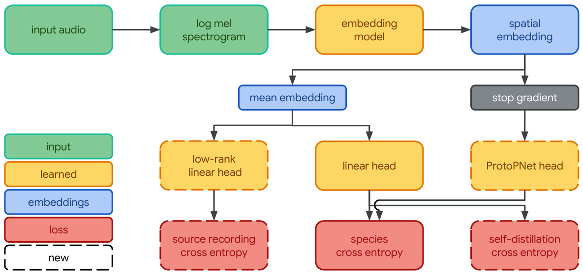
Figure 1: Perch 2.0 employs EfficientNet-B3 architecture with multi-task learning heads for species classification and source prediction

Introduction to Bioacoustics Breakthrough
The field of bioacoustics has undergone a paradigm shift with the release of Perch 2.0 by Google DeepMind. This advanced model demonstrates how simple supervised learning approaches can outperform complex self-supervised methods in analyzing animal sounds. Let’s explore how this technology works and why it matters for ecological monitoring.
Understanding Perch 2.0’s Technical Foundation
Core Architecture Components
-
Frontend Processing
Converts 5-second audio clips into log mel-spectrograms using:-
32 kHz sampling rate -
10 ms hop length -
20 ms window length -
128 mel-scaled frequency bins (60 Hz – 16 kHz range)
-
-
EfficientNet-B3 Backbone
A compact 12-million parameter convolutional neural network that:-
Processes time-frequency representations -
Generates 1536-dimensional embeddings -
Operates efficiently on consumer hardware
-
-
Multi-Head Output System
Three parallel classifiers work together:-
Linear classifier for species prediction -
Prototype learning classifier for interpretability -
Source prediction head for self-supervision
-
Figure 2: System diagram showing audio windowing and feature extraction process

Key Innovations in Training Methodology
1. Expanded Training Data
The model was trained on 1.54 million audio clips from diverse sources:
-
Xeno-Canto: 860k bird recordings -
iNaturalist: 480k wildlife recordings -
Tierstimmenarchiv: 26k animal sounds -
FSD50K: 40k environmental sounds
2. Advanced Data Augmentation
A novel mixup technique creates composite training samples by:
-
Mixing 2-5 audio segments -
Using Dirichlet distribution for weight allocation -
Preserving signal power through normalization -
Creating multi-label targets instead of weighted averages
3. Self-Distillation Framework
The training process involves two phases:
-
Prototype Training: -
Train a prototype-based classifier -
Use its predictions as soft targets
-
-
Distillation Phase: -
Freeze prototype weights -
Train linear classifier using soft targets -
Achieve 0.9% AUC improvement over baseline
-
Benchmark Performance Results
BirdSet Benchmark (6 North American Soundscapes)
| Metric | Perch 1.0 | Perch 2.0 (Random) |
|---|---|---|
| ROC-AUC | 0.839 | 0.908 |
| Top-1 Accuracy | 0.613 | 0.665 |
BEANS Cross-Taxa Benchmark
| Task Type | Perch 1.0 | Perch 2.0 (PP) |
|---|---|---|
| Classification | 0.809 | 0.840 |
| Detection (mAP) | 0.353 | 0.502 |
Marine Transfer Learning Breakthrough
Despite minimal marine training data, Perch 2.0 outperforms specialized models:
| Dataset | Perch 1.0 | Perch 2.0 | Multispecies Whale |
|---|---|---|---|
| DCLDE 2026 | 0.968 | 0.977 | 0.954 |
| NOAA PIPAN | 0.905 | 0.924 | 0.917* |
| ReefSet | 0.970 | 0.981 | 0.986* |
*Indicates model was trained on target dataset
Practical Applications & Implementation
Key Advantages
-
Zero-Shot Capability
Works immediately on new species without retraining -
Hardware Efficiency
Processes 5-second clips in <5 seconds on consumer GPUs -
Flexible Input Handling
Accepts:-
Audio files (WAV/MP3) -
PDF documents with embedded audio -
Image files of spectrograms -
URL links to media resources
-
Recommended Workflow
-
Preprocessing
Convert long recordings to 5-second windows using:def preprocess_audio(audio_path): # Implement 5s windowing with 2.5s stride # Return list of windowed samples -
Embedding Generation
Extract 1536-dimensional features:embeddings = model.encode(audio_windows) -
Downstream Tasks
Apply to:-
Species identification -
Population monitoring -
Soundscape analysis -
Individual vocalization tracking
-
FAQ: Technical Implementation Guide
Q1: How to handle variable-length recordings?
A: Split into 5-second windows with 50% overlap. For recordings <5s, pad with zeros before processing.
Q2: What hardware is required?
A: Minimum requirements:
-
4GB VRAM (RTX 3050 equivalent) -
8GB RAM -
2.5GHz quad-core CPU
Q3: How to integrate with existing systems?
A: Use REST API endpoints:
import requests

response = requests.post(
    "https://api.perch2.com/predict",
    files={"audio": open("recording.wav", "rb")},
    headers={"Authorization": "Bearer API_KEY"}
)
Q4: How to interpret confidence scores?
A: Use thresholding:
-
0.9: High confidence species detection
-
0.7-0.9: Possible detection (manual verification recommended) -
<0.7: Insufficient evidence
Future Development Directions
-
Semi-Supervised Learning
Leverage source prediction task to incorporate unlabeled data from rare species -
Dynamic Soundscape Analysis
Combine with satellite tracking for migration pattern studies -
Acoustic Feature Visualization
Develop prototype-based explanation tools for bioacousticians
Conclusion
Perch 2.0 demonstrates that well-designed supervised models can achieve state-of-the-art results in bioacoustics without requiring massive unlabeled datasets. Its efficient architecture and strong transfer learning capabilities make it particularly valuable for conservation applications where computational resources are limited.