Building a Fast, Memory-Efficient Hash Table in Java: A Deep Dive into SwissTable-Inspired Design

Have you ever wondered why some hash tables remain lightning-fast even under high load, while others slow to a crawl as they fill up? One day, I stumbled upon SwissTable—a design that made me squint, grin, and immediately regret every naive linear-probing hash table I’d ever written.

This post is the story of how I tried to bring that “why is this so fast?” feeling into the Java world. It’s part technical deep dive, part engineering diary, and part cautionary tale about performance optimization work. I’ll walk you through the core ideas behind SwissTable, show how it became standard in languages like Rust and Go, and share in detail the process, challenges, and lessons learned from implementing a similar structure in Java.

1. The “Aha!” Moment: Understanding SwissTable

SwissTable originated from Google’s work, initially presented as a new C++ hash table approach and later integrated into the Abseil library. At its heart, it still does the usual hash table work: compute hash(key), pick a starting slot, and probe until you find your key or an empty slot.

The twist lies in separating metadata (tiny “control bytes”) from the actual key-value storage and using these control bytes to avoid expensive key comparisons most of the time. Instead of immediately dereferencing a bunch of keys—which are likely cold in cache and often pointer-heavy—it first scans a compact array of control bytes. This array is dense, cache-friendly, and easy to compare in bulk. If this sounds like a tiny Bloom filter, you’re on the right track: the control bytes act as a cheap “maybe” gate before we pay the cost of real key comparisons.

To make probing cheap, SwissTable effectively splits the hash into two parts: h1 and h2. Think of h1 as selecting where to start probing (which group to look at first), and h2 as a small fingerprint stored in the control byte to quickly rule slots in or out. It’s not a full hash—just enough bits to filter candidates before touching the actual keys.

So during a lookup, you compute the hash, derive (h1, h2), jump to the group indicated by h1, and compare h2 against all control bytes in that group before looking at any keys. This means most misses (and many hits) avoid accessing key memory entirely until the metadata signals, “There’s a plausible candidate here.”

Because probing stays cheap, SwissTable can tolerate much higher load factors—up to about 87.5% (7/8) in implementations like Abseil’s flat_hash_map—without falling off a performance cliff, directly improving memory efficiency. The net result is a design that is both faster (fewer cache misses, fewer key compares) and more compact (higher load factor, fewer side structures like overflow buckets).

2. From Concept to Standard: The SwissTable Journey Across Languages

You know a design is generational when it stops being a cool library trick and starts showing up in standard libraries.

Starting with Rust 1.36.0, std::collections::HashMap switched to the SwissTable-based hashbrown implementation. It’s described as using quadratic probing and SIMD lookup, which is essentially SwissTable in spirit and technique. That was my “okay, this isn’t niche anymore” moment.

Then Go joined the party: Go 1.24 ships a new built-in map implementation based on the SwissTable design, straight from the Go team’s own blog post. Their microbenchmarks report map operations to be up to 60% faster than Go 1.23, and full application benchmarks show about a 1.5% geometric-mean improvement in CPU time. For a practical “this matters in real systems” story, see Datadog’s write-up on how Go 1.24’s SwissTable-based maps and their new layout and growth strategy translate into serious memory savings at scale.

At that point, SwissTable stopped feeling like a “clever C++ trick” and started feeling like the modern baseline. I couldn’t shake the thought: Rust did it, Go shipped it… so why not Java? With modern CPUs, a strong JIT, and the Vector API finally within reach, it felt less like a technical impossibility and more like an itch I had to scratch.

And so, I fell down the rabbit hole.

3. When SwissTable’s Secret Sauce Meets the Java Vector API

A big part of SwissTable’s speed comes from doing comparisons wide: checking many control bytes at once instead of looping byte-by-byte and branching constantly. That’s exactly the kind of workload SIMD excels at: load a small block, compare against a broadcasted value, get a bitmask of matches, and only then branch into “slow path” key comparisons. In other words, SwissTable isn’t just “open addressing done well”—it’s “open addressing shaped to fit modern CPUs.”

Historically, doing this portably in Java was awkward: you either trusted auto-vectorization, used Unsafe, wrote JNI, or accepted the scalar loop. But the Vector API has been incubating specifically to let Java express vector computations that reliably compile down to good SIMD instructions on supported CPUs.

In Java 25, the Vector API is still incubating under jdk.incubator.vector. For me, the important question wasn’t “is it final?” but “is it usable enough to express the SwissTable control-byte scan cleanly?” Because if I can write “compare 16 bytes, produce a mask, act on set bits” in plain Java, the rest of SwissTable becomes mostly careful data layout and resizing logic. Once you see the control-byte scan as the hot path, you start designing everything else to make that scan cheap and predictable.

So yes: the Vector API was the permission slip I needed to try something I’d normally dismiss as “too low-level for Java.”

4. The Implementation Journey: What Java Makes Easy vs. Hard

I started with the core SwissTable separation: a compact control array plus separate key/value storage. The control bytes are the main character—if they stay hot in cache and the scan remains branch-light, the table feels fast even before micro-optimizations.

I used the familiar h1/h2 split: h1 selects the initial group, while h2 is the small fingerprint stored in the control byte to filter candidates. Lookup became a two-stage pipeline: (1) vector-scan the control bytes for h2 matches, (2) for each match, compare the actual key to confirm. Insertion reused the same scan, but added a “find first empty slot” path once we knew the key didn’t already exist.

Where Java started pushing back was layout realism.

In C++, you can pack keys/values tightly; in Java, object references mean the “key array” is still an array of pointers, and touching keys can still trigger a parade of cache misses. So the design goal became: touch keys as late as possible, and when you must touch them, touch as few as possible—the SwissTable philosophy applied to Java’s reality.

Deletion required tombstones (a “deleted but not empty” marker) so probing chains wouldn’t break, but tombstones also accumulate and can quietly degrade performance if never cleaned up.

Resizing was its own mini-project: a full rehash is expensive, but clever growth strategies (like Go’s use of table splitting/extendible hashing) show how far you can go if you’re willing to complicate the design.

I also had to treat the Vector API as an optimization tool, not a magic wand. Vector code is sensitive to how you load bytes, handle tails, and whether the JIT can keep the loop structure stable. I ended up writing the control-byte scan as a very explicit “load → compare → mask → iterate matches” loop.

At this stage, the prototype already worked, but it wasn’t yet “SwissTable fast”—it was “promising, and now the real work begins.”

5. The Pieces of SwissMap That Actually Mattered

Here’s what survived the usual round of “this feels clever but isn’t fast” refactors.

5.1 Control Bytes & Layout

With non-primitive keys, the real cost is rarely “a few extra byte reads”—it’s pointer chasing. Even one equals() call can walk cold objects and pay cache-miss latency. So SwissMap treats the control array as the first line of defense: scan a tight, cache-friendly byte array to narrow the search to a handful of plausible slots before touching any keys/values.

This matters even more in Java because “keys/values” usually means arrays of references. On 64-bit JVMs, compressed oops (often enabled up to ~32GB depending on alignment/JVM flags) pack references into 32 bits, making reference arrays denser. When compressed oops is off, references widen to 64 bits, and the same number of key touches can spill across more cache lines.

Either way, the control array does most of the work: most misses die in metadata. Compressed oops just makes the unavoidable key touches cheaper when they do happen.

5.2 Load Factor

In classic open addressing, pushing the load factor up usually means the average probe chain length increases rapidly—more branches, more random memory touches, and a steep cliff in miss cost. That’s why many general-purpose hash maps pick conservative defaults. Java’s HashMap, for example, defaults to a 0.75 load factor to keep miss costs from ballooning as the table fills.

SwissTable flips the cost model: probing is dominated by first scanning the control bytes, which are dense, cache-friendly, and cheap to compare in bulk. This means “one more probe group” is often just one more control-vector load + compare, not a bunch of key equals() calls. With SwissTable-style probing, the table can run denser without falling off a cliff. Abseil’s SwissTable-family maps are well known for targeting a ~7/8 (0.875) maximum load factor; even when the table is crowded, most probes are still “just metadata work.”

That trade-off is exactly what I wanted in Java too: higher load factor → fewer slots → smaller key/value arrays → fewer cache lines touched per operation, as long as the control scan stays the fast path.

5.3 Sentinel Padding

SIMD wants fixed-width loads: 16 or 32 control bytes at a time. The annoying part is the tail—the last group near the end of the control array. In native code, you might “over-read” a few bytes and rely on adjacent memory being harmless. In Java, you don’t have that luxury: out-of-bounds is a hard stop.

Without padding, the probe loop needs tail handling: extra bounds checks, masked loads, or end-of-array branches—exactly the kind of bookkeeping you don’t want in the hottest path. Adding a small sentinel padding region at the end of the array lets every probe issue the same vector load, keeping the loop predictable and JIT-friendly.

5.4 H1/H2 Split

Split the hash into h1 (which selects the starting group) and h2 (a small fingerprint stored per slot in the control byte). h1 drives the probe sequence (usually via a power-of-two mask), while h2 is a cheap first-stage filter: SIMD-compare h2 against an entire group of control bytes and only touch keys for the matching lanes.

SwissMap uses 7 bits for h2, leaving the remaining control-byte values for special states like EMPTY and DELETED. That’s the neat trick: one byte answers both:

• “Is this slot full/empty/deleted?”
• “Is this slot even worth a key compare?”

Most lookups reject non-matches in the control plane. And if a probed group contains an EMPTY, that’s a definitive stop signal: the probe chain was never continued past that point, so the key can’t exist “later.”

5.5 Reusing the Loaded Control Vector

A ByteVector load isn’t free—it’s a real SIMD-width memory load of control bytes. On my test machine, that load alone was ~6ns per probed group. In a hash table where a get() might take only a few dozen nanoseconds, that’s a meaningful tax.

So SwissMap tries hard to load the control vector exactly once per group and reuse it:

• Use the same loaded vector for the h2 equality mask (candidate lanes)
• And again for the EMPTY/DELETED masks (stop/continue decisions)

No extra passes, no “just load it again,” no duplicate work.

5.6 Tombstones and Deletion Management

Deletion is where correctness bites in open addressing: if you mark a removed slot as EMPTY, you can break the probe chain. Keys inserted later in that chain would become “invisible” because lookups stop at the first empty.

Tombstones solve this by marking the slot as DELETED (“deleted but not empty”), so lookups keep probing past it.

On put, tombstones aren’t just a correctness hack—they’re also reusable space. The common pattern is:

• During probing, remember the first DELETED slot you see
• Keep probing until you either find the key (update) or hit an EMPTY (definitive miss)
• If the key wasn’t found, insert into the remembered tombstone rather than the later empty slot

This tends to keep probe chains from getting longer over time, reduces resize pressure, and prevents workloads with lots of remove/put cycles from slowly poisoning performance.

5.7 Triggering a Same-Capacity Rehash

Tombstones preserve correctness, but they dilute the strongest early-exit signal: EMPTY. A table with many DELETED slots tends to probe farther on misses and inserts—more control scans, more vector loads, and more chances to touch cold keys.

So SwissMap tracks tombstones and triggers a same-capacity rehash when they cross a threshold (as a fraction of capacity or relative to live entries). This rebuilds the control array, turning DELETED back into EMPTY and restoring short probe chains—basically compaction without changing logical contents.

5.8 A Resize Rehash Without Redundant Checks

Resizing forces a rehash because h1 depends on capacity. The obvious approach is “iterate old entries and call put into the new table,” but that pays for work you don’t need: duplicate checks, extra branching, and unnecessary key equality calls.

The faster path treats resize as a pure move:

• Allocate fresh control/key/value arrays
• Reset counters
• Scan the old table once, and for each FULL slot:

  • Recompute (h1, h2) for the new capacity
  • Insert into the first available slot found by the same control-byte probe loop
  • Without checking “does this key already exist?” (it can’t: you’re moving unique keys)

This makes resizing a predictable linear pass over memory rather than a branchy series of full put() operations.

5.9 Iterators Without Extra Buffers

Iteration is another place where “simple” becomes surprisingly expensive. You can scan linearly and yield FULL slots, but many designs want a stable-ish visit pattern without allocating a separate dense list. Some reinsertion/rehash interactions can even go accidentally quadratic (see the Rust iteration write-up).

SwissMap avoids extra buffers by iterating with a modular stepping permutation: pick a start and an odd step (with power-of-two capacity, any odd step is coprime), then visit indices via repeated idx = (idx + step) & mask. This hits every slot exactly once, spreads accesses across the table, and keeps iteration as a tight loop over the same control-byte state machine used elsewhere.

Here’s a trimmed version of the lookup method showing how the probe loop hangs together around the control bytes:

protected int findIndex(Object key) {
    if (size == 0) return -1;
    int h = hash(key);
    int h1 = h1(h);
    byte h2 = h2(h);
    int nGroups = numGroups();
    int visitedGroups = 0;
    int mask = nGroups - 1;
    int g = h1 & mask; // optimized modulo operation (same as h1 % nGroups)
    for (;;) {
        int base = g * DEFAULT_GROUP_SIZE;
        ByteVector v = loadCtrlVector(base);
        long eqMask = v.eq(h2).toLong();
        while (eqMask != 0) {
            int bit = Long.numberOfTrailingZeros(eqMask);
            int idx = base + bit;
            if (Objects.equals(keys[idx], key)) { // found
                return idx;
            }
            eqMask &= eqMask - 1; // clear LSB
        }
        long emptyMask = v.eq(EMPTY).toLong(); // reuse loaded vector
        if (emptyMask != 0) { // any empty in a probed group is a definitive miss in SwissTable-style probing
            return -1;
        }
        if (++visitedGroups >= nGroups) { // guard against infinite probe when table is full of tombstones
            return -1;
        }
        g = (g + 1) & mask;
    }
}

6. Performance Benchmarks

I didn’t want to cherry-pick numbers that only look good on synthetic cases.
So I used a simple, repeatable JMH setup that stresses high-load probing and pointer-heavy keys—the exact situation SwissTable-style designs are meant to handle.

All benchmarks were run on Windows 11 (x64) with Eclipse Temurin JDK 21.0.9, on an AMD Ryzen 5 5600 (6C/12T).

For context, I compared against HashMap, fastutil’s Object2ObjectOpenHashMap, and Eclipse Collections’ UnifiedMap.

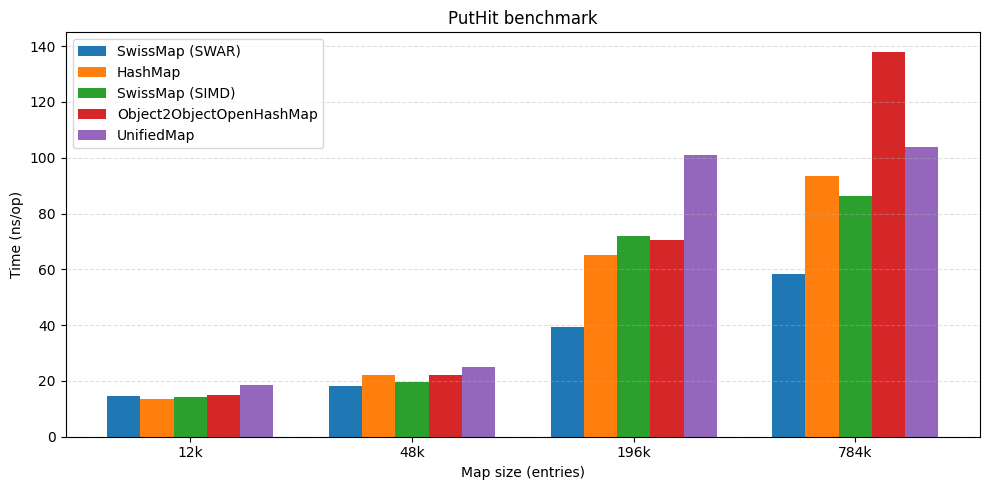
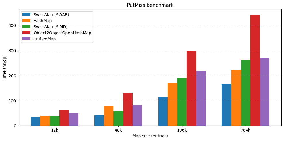
6.1 The Headline Results

At high load factors, SwissMap maintains competitive throughput against other open-addressing tables and stays close to JDK HashMap performance. In some benchmarks, it comes out ahead by a significant margin.

put hit performance	put miss performance

get hit performance	get miss performance

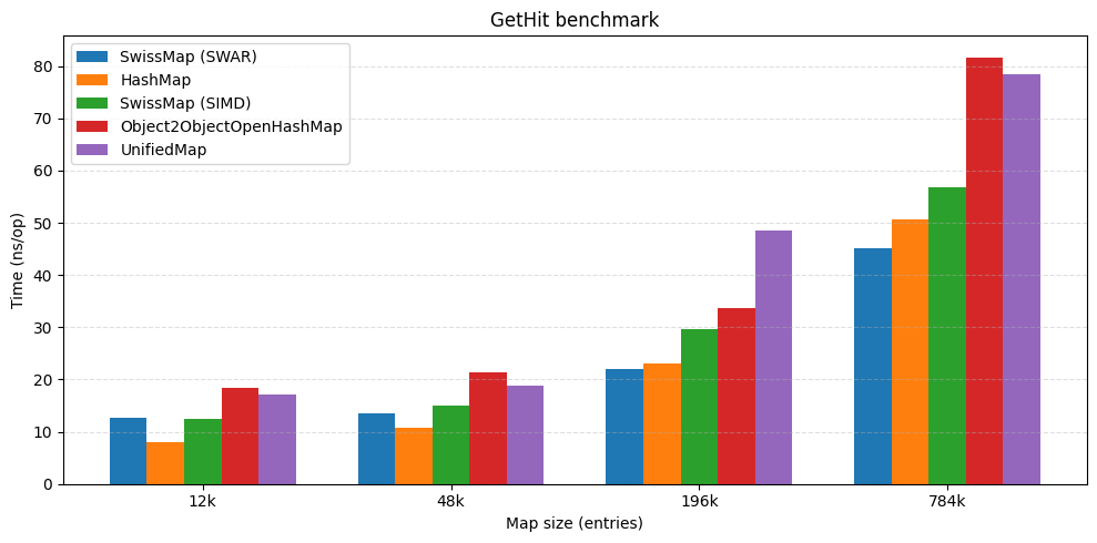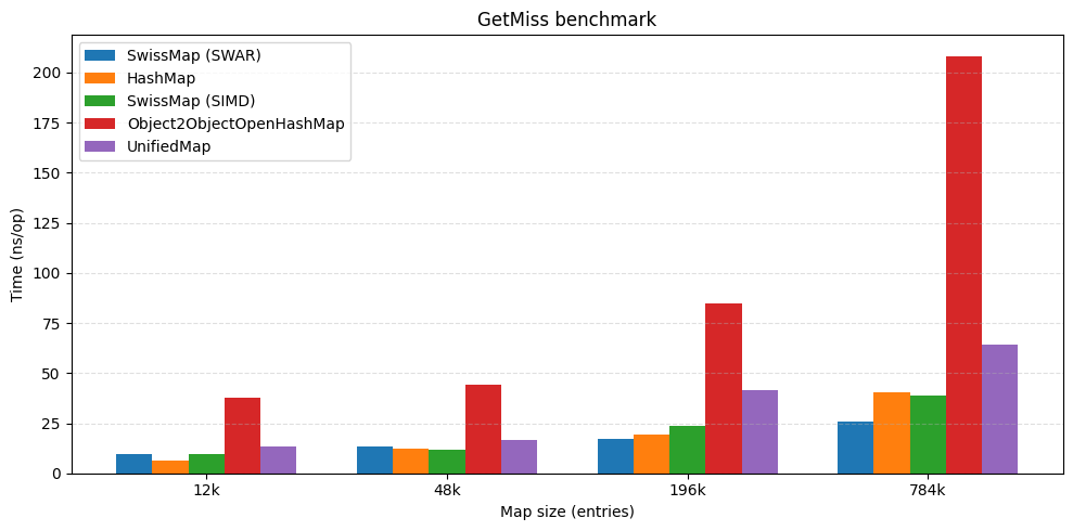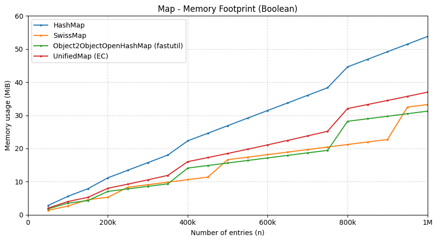
On memory, the flat layout (no buckets/overflow nodes) plus a 0.875 (7/8) max load factor translated to a noticeably smaller retained heap in small-payload scenarios—over 50% less than HashMap in this project’s measurements.

6.2 Caveat

These numbers are pre-release; the Vector API is still incubating, and the table is tuned for high-load, reference-key workloads. Expect different results with primitive-specialized maps or low-load-factor configurations.

7. Quick Heads-Up: About the SWAR Variant

You might notice a SWAR-style SwissTable variant appearing out of nowhere in the benchmark section. That version is part of a follow-up round of tuning: same SwissTable control-byte workflow, but implemented with SWAR to reduce overhead and avoid leaning on the incubating Vector API.

If SWAR is new to you, think of it as “SIMD within a register”: instead of using vector lanes, we pack multiple control bytes into a single 64-bit word and do the same kind of byte-wise comparisons with plain scalar instructions. The end result is a similar fast-path idea, just expressed in a more portable (and JDK-version-friendly) way.

I didn’t want this post to turn into three posts, so I’m saving the full “how/why” (SWAR included) for the next write-up—stay tuned.

8. Frequently Asked Questions (FAQ)

1. What’s the main difference between SwissTable and the traditional Java HashMap?
The traditional HashMap uses separate chaining (array + linked list/red-black tree), while SwissTable (and its Java implementation SwissMap) uses open addressing and separates metadata (control bytes) from data storage. The core difference lies in the lookup path: SwissMap first performs a fast SIMD scan over a dense control-byte array; only matching candidates need to access the actual key objects, dramatically reducing cache misses and expensive equals() calls.

2. Why can the load factor be set as high as 0.875?
Because the performance bottleneck shifts. In traditional open addressing, a high load factor leads to long probe chains, meaning many key comparisons and branches. SwissTable’s probing cost is dominated by SIMD-scanning the control bytes, which is very fast. Therefore, even when the table is very full, most probe operations are just manipulating metadata in a small, hot cache region, resulting in a gentler performance degradation curve.

3. Is the Vector API mandatory?
For implementing the SIMD-accelerated control-byte scan, using the Vector API is currently the clearest and most forward-looking approach in Java. However, as mentioned, you can also use SWAR (SIMD Within A Register) techniques to achieve similar acceleration without relying on the incubating API, trading some flexibility for better compatibility.

4. Don’t tombstones cause performance degradation?
Yes, if they accumulate too much. While tombstones maintain correctness, they lengthen probe chains (because lookups don’t stop at DELETED). Therefore, SwissMap needs to monitor the tombstone count and trigger a “same-capacity rehash” to clean them up when a threshold is crossed—essentially an internal compaction operation.

5. Is this implementation production-ready?
The implementation discussed here is experimental (the HashSmith project). It’s for exploring design ideas and running benchmarks. While it borrows from mature designs, putting it into production would require more comprehensive consideration of edge cases, concurrency support, serialization, etc. However, its core ideas (separating metadata, SIMD scanning, high load factor) are directly instructive for optimizing hash table usage in high-performance Java applications.

6. Are there any special requirements for key objects?
As with any hash table, keys must correctly implement hashCode() and equals() methods. Since SwissMap heavily relies on the hash value to generate h1 and h2, a well-distributed hashCode() is crucial for performance.

9. Key Takeaways and Conclusion

This journey of bringing SwissTable ideas into Java clearly highlights several key trends in modern high-performance hash table design:

1. Trade Computation for Access, Metadata First: Increase a small amount of computation (like splitting the hash, SIMD comparison) to drastically reduce random memory accesses to main data, especially cache-unfriendly pointer chasing. This is the core of performance gains.
2. Design for Cache and Vectorization: Data layout (separating control bytes from data, dense packing) is optimized directly for CPU cache hierarchy and SIMD instructions, turning the hottest path into a linear, predictable memory access pattern.
3. Re-evaluate Trade-offs: By changing the cost model (making probing cheap), you can break traditional constraints (like load factor limits), achieving gains in both memory efficiency and runtime performance.
4. Leverage and Challenge Language Features: Java’s Vector API opens the door for expressing such algorithms, but the language’s own characteristics (like object headers, reference arrays) also introduce unique challenges, requiring tailored optimization strategies (like leveraging compressed pointers).

This endeavor also reminds us that performance optimization work is often a process of delving into details, constant measurement, and testing. An elegant conceptual design must confront the practical constraints of specific platforms and language environments in its implementation.

10. Resources and Next Steps

If you’re interested in the code, benchmark details, or experimenting yourself, check out this public experiment: HashSmith. It includes SwissMap as well as a SwissSet variant, along with JMH benchmarks and documentation.

For a deeper understanding of the original SwissTable design, I highly recommend watching Google engineer Matt Kulukundis’s CppCon talk: CppCon talk on SwissTable. It’s clear, practical, and packed with details that make the design click.

I hope this in-depth exploration provides you with valuable insights into hash table performance optimization and modern Java performance programming. Whether you’re looking to build more efficient data structures for specific scenarios or to better understand the internals of the tools you use, this kind of exploration is highly beneficial.